Spatial Analysis

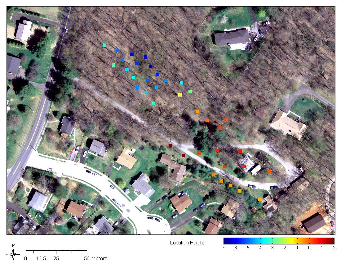
We begin by looking at two months of data (Jun 2009- Aug 2009) for the summer at depth 1. The heat map below shows the soil temperature values for different locations in the Cub Hill deployment. The figure below also shows the locations of the sensors that are given the forest and grass tags. The vectors are organized using the angle between data from each location of the median vector in ascending order.

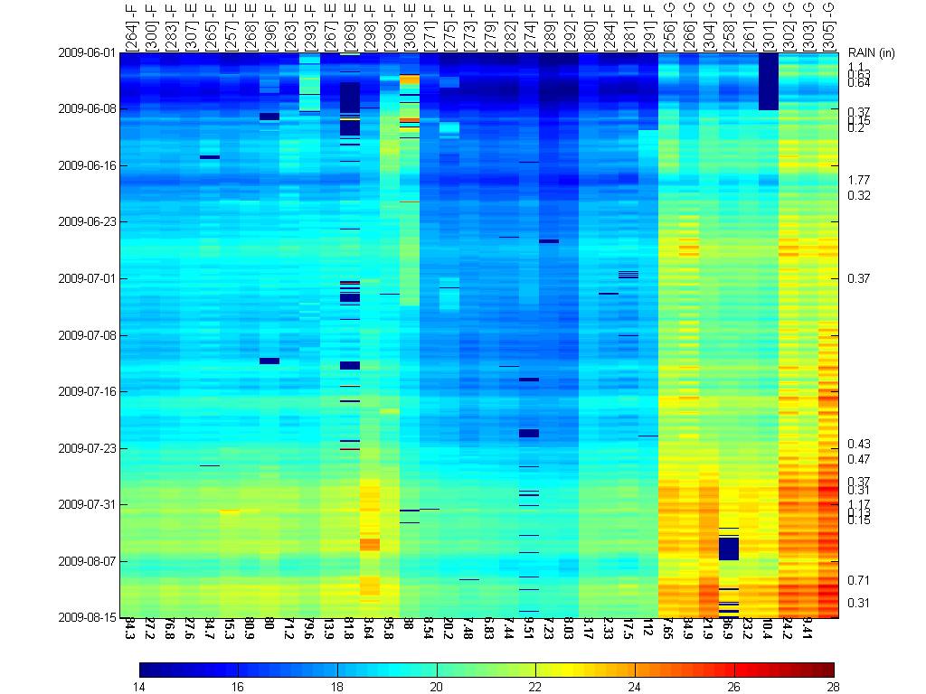
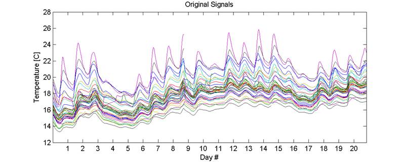
The figure below shows the raw time signals for June 1, 2009 to Aug 1, 2009. Out of 50 locations, around 10 locations have a lot of missing values and noise so they and were removed from this analysis. The raw time signals for the first 20 days are shown in the figure below.

The figure below shows the first 20 days of the raw signals. Next, we remove the ramp value for each daily vector. The last panel shows the residuals after removing the first 2 principal components using the basis shown above.

The median value of the variogram at a given distance is shown in the figure below. The figure also shows the number of samples using which the median was calculated.

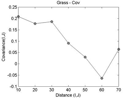
The correlogram for the same dataset is shown below too

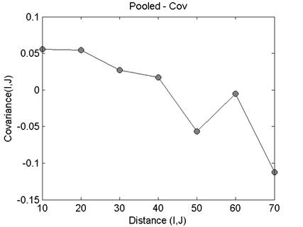
I also tried the variogram and correlogram on the projection on the third PC. The figure is shown below.