GALEX photometry tests

Approach

It has been decided at the recent JHU meeting to look a bit further at some photometry properties of the GALEX fields to see if effects as zero-point variations, for instance, could explain the peculiar behaviour of the Angular Correlation Function (ACF), when all fields are used at the same time.
A first approach is to look at objects observed several times by GALEX in the overlap regions between fields. This method has however some limitations, as it focuses on field edges where the photometry accuracy decreases, and the use of a conservative cut radius reduces significantly the number of objects.
We tried another statistical approach, which enables to use most of the objects in the fields, and which is independent of the number of objects. Our tests rely on a statistical tool called the Mann-Whitney test (Wikipedia article) . This test can be used to decide if two sets are drawn from the same distribution. On practice, the output of this test is the probability that this is actually the case.

Method

We consider GR3 MIS fields, using:

FUV or NUV exposure times greater than 1000s.
Objects within the primary resolution and with fov_radius < 0.5 deg
Objects with UV magnitudes: 17 < UV < 22
Objects with SDSS galaxies (type = 3) counterparts, to avoid any effects due to variation of stars counts with Galactic latitude.

For each field, we build a test sample, from the magnitudes of all objects that meet these criterion; we build also the control sample, from the magnitudes of all objects meeting the criterion in all other fields. We perform the Mann-Whitney test for each field using these inputs. Hence we derive for each field the probability that the magnitude distribution of this field is drawn from the same distribution than the overall sample.

Results

Field classification

The following plots show the histogram of the p-value from the Mann-Whitney test (left:FUV selection; right: NUV selection). The dashed line shows the 0.05 confidence level; we use this threshold to decide if fields are drawn from the same distribution than the overall sample. According to these tests, for the FUV selection, there is 25% of the fields that are not drawn from the same distribution (45% for NUV).

Mann-Whitney test p-value histogram for FUV selection

Mann-Whitney test p-value histogram for NUV selection

There are no obvious trends between the result of the Mann-Whitney test and the mean galactic extinction in the fields, or the mean background (same trends in NUV).

ACF

We computed the ACF of the GR3 MIS fields, for various cuts in the p-value of the Mann-Whitney test. We used only the 'Combined fields method' for the ACF computation, which uses all fields at once. Combined field ACFs for UV<22

Each plot shows the ACF as a function of the angular scale. The right hand side plots show results for the FUV selection, left ones for NUV selection. The blue (solid line) ACF was obtained from all the fields; the green (dotted line) from fields with p-value > 0.05 (fields drawn from the same distribution than the overall sample); the purple (dashed line) from fields with p-value < 0.05 (fields not drawn from the same distribution than the overall sample) and finally in red (dot-dashed line), we show the ACF from fields with p-value < 0.01 (likely to be worse than the previous ones). There are 3 double-plots, for UV < 22 (top), UV < 21.5 (middle) and UV < 21 (bottom).

These figures show that there is a clear trend of the amplitude (and slope as well) of the ACF with the p-value from the Mann-Whitney test: the amplitude (slope) increases (decreases) when p decreases. There is a flattening of the ACF at scales larger than 0.1 degrees, which is more important at brighter magnitudes. The discrepancy of the ACFs is less severe in NUV: there is for instance no difference between the various ACFs at NUV < 22, but there are at brighter magnitudes.

From these figures, it is obvious that this simple statistical tool enables to find fields that are problematic regarding to clustering measurements. A quick visual inspection of a few images of the fields with p < 0.05 suggests that there is no obvious pattern linking these fields: some show cirrus, or artifacts (horseshoes), or nothing ...

Varying the zero-point

We tried to see if we can improve the ACFs results of the fields with p-values < 0.05 assuming a simple zero-point change. We allow the zero-point to vary between -0.5 and 0.5, apply it and perform the Mann-Whitney test. We choose the best zero-point variation as the one corresponding to the largest p-value.

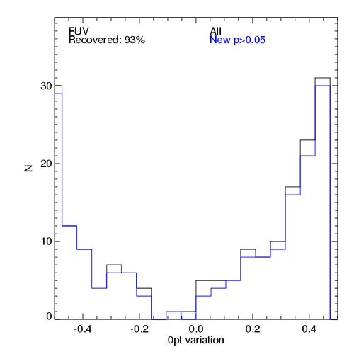
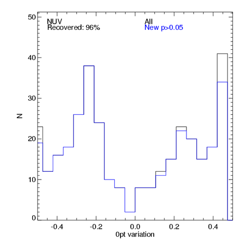
The following plots show the histograms of the best zero-point variation according to this test. The black histogram represents all fields; the blue one show only the fields that we can recover, that is the fields that get a p-value > 0.05 after the zero-point variation. Left is for FUV, right for NUV. This method enables to recover most of the fields in both cases (fraction recovered > 90%). Of course, this does not mean that the origin of the discrepancy in the photometry for these fields is only solved by a zero-point variation.

Histogram of best zero-point variation according to Mann-Whitney test

This is obvious when we inspect the ACFs of the fields with these zero-point applied. Combined field ACFs for UV<22 with 0point variation for fields with p<0.05

Combined field ACFs for UV<22 with 0point variation for fields with p<0.05

Combined field ACFs for UV<21.5 with 0point variation for fields with p<0.05

Combined field ACFs for UV<21 with 0point variation for fields with p<0.05

These plots show some same ACFs as before: blue (solid) represents the ACF of the fields that have a p-value > 0.05; green (dotted) the ACFs of the fields that have a p-value < 0.05. The comparison of the two last ACFs enables to see how we can correct for the effects seen here with a simple zero-point variation: we selected the fields with a p-value < 0.05, and that require a zero point variation between -0.2 and 0.2 (in order to restrict to relatively low zero-point shifts). We computed the ACFs of these fields using the pipeline magnitudes (purple, dashed ACF), and applying our zero-point shift (red, dot-dashed).
At this point, note that the number of fields that make the red and purple ACFs is lower than the number of fields that make the green. This means that the geometry of the sample is quite different, resulting in less cross-fields galaxy pairs, and then to a larger Integral Constraint bias (which yields a loss of power at large scales). Hence the purple and red ACFs can be compared directly with each other, but not directly with the green and blue.
These results show that a simple zero-point variation is not sufficient to get rid of the effects we observe. The impact of a zero-point variation is actually worse at faint magnitudes.